
Use Case: Dynamic Controller Placement
Introduction
This use case is an example for a general category of use cases related to the migration of Virtual Network Functions. Here the network functions are SDN controllers running in a virtual machine. Compared to so many controller placement works, for a meaningful flexibility measurement, we focus on the control plane dynamics to react to varying network situations (e.g. load). Therefore, we have accurately modeled the controller migration dynamics with (a) controller(s) migration and (b) switch(es)-to-controller reassignment, i.e., a complex function chain.
We consider the following scenario. For more details see [1].
- Scenario: Dynamic SDN control plane that can adapt its configuration (location of controller(s) and switch-to-controller assignment) to changing traffic flows to achieve an optimal control performance
- Objective: Optimal control performance in term of the average flow setup time, i.e., the time involved to detect a new flow by the controller and to setup the flow rules on all switches on its path.
- Network topology: Abilene network
- Different system to compare for flexibility: number of SDN controllers (1 to 4)
- Flexibility aspect: Function placement
- Request (input to flexibility evaluation): flow arrival (from distribution)
- Flexibility measure: Fraction of successful controller placements
- Time threshold T: is varied between 120 ms and 250 ms
- Cost threshold C: is not considered, but recoded in a separate plot
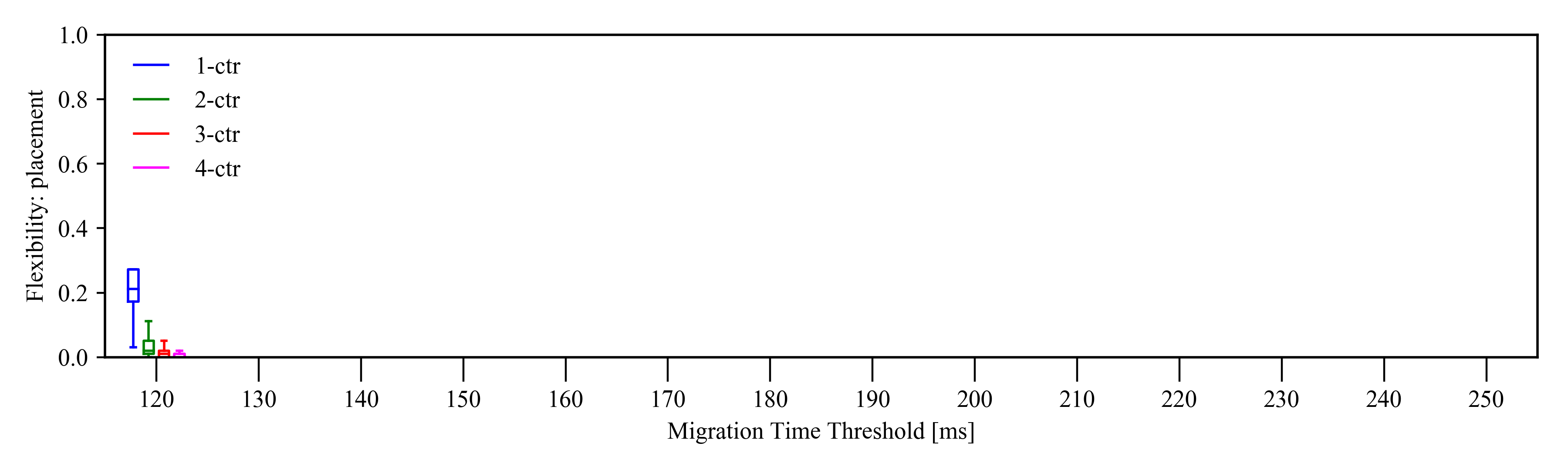
Flexibility
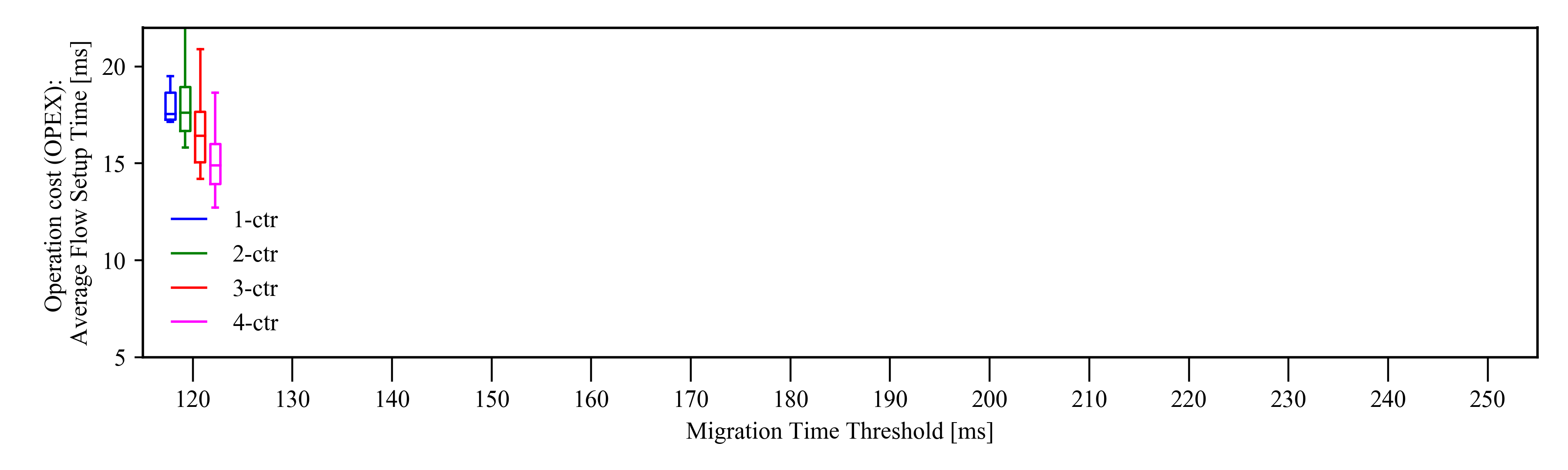
Cost
Observations explained (from [1])
Network Flexibility- General trend: flexibility increases with increasing T, no matter how many controllers are deployed. This follows our intuition that larger T ensures that more reconfigurations can be fulfilled.
- Counter intuitive: For smaller T, the flexibility exhibited by one controller (1-ctr) is higher than that of more controllers. This is because there is a high chance that the single controller does not need to change its configuration to achieve its optimal performance.
- Multiple controllers: the system tends to result in new optimal placements, that require more reconfigurations to be done within T. Hence, only at larger T, the flexibility measure increases with the number of controllers.
- General trend: higher cost emerges if T cannot be fulfilled by the migration process, where the new optimal placement will be discarded and the average flow setup time will be degraded.
- More controllers available: the system cost decreases as flexibility increases with larger T. For example, the average flow setup time of 4-ctr drops from 15 ms to less than 10 ms, which is a 30% decrease in cost.
- For 1-ctr case: even if the flexibility increases with larger T up to almost 90% of the requests, the cost improvement is marginal.
References
- W. Kellerer and A. Basta and P. Babarczi and A. Blenk and M. He and M. Klügel and A. M. Alba, "How to Measure Network Flexibility? A Proposal for Evaluating Softwarized Networks," in IEEE Communications Magazine, vol. 56, no. 10, pp. 186-192, October 2018.
Use Case: Resilience
Introduction
This use case is an example for a category of uses cases related to the routing of flows in a network system reacting to events. Here routing reacts to link failures. We illustrate the network flexibility of different routing methods, including purely reactive systems and systems where the resilience to failures is proactively pre-planned (protection).
Note that in this use case, we are able to measure network flexibility with a complete set of challenges (= requests) as we measure the recovery success rate for all possible connections (all source-destination pairs) exposed to all possible single and link-pair failures, hence we do not draw the challenges from a distribution.
We consider the following scenario. For more details see [1].
- Scenario: SDN-based network … is exposed to single link and link-pair failures and is reacting to recover those failures
- Objective: recovery of connections between all possible source-target pairs
- Network topology: varied
- Different system to compare for flexibility routing methods (1+1, 1:1, Restoration)
Remember, network flexibility of a flow routing method represents its ability to respond to network failures under a recovery time threshold T and a cost threshold C.
- Flexibility aspect: flow configuration
- Request: (input to flexibility evaluation) varied - (all) possible single and link-pair values
- Time threshold T: is varied between 0 ms and 100 ms
- Cost threshold C: is not considered, but recorded
A failure request is not supported if the time it takes to recover the failure is larger than T. A failure request is supported if the normal operation can be restored within T. An evaluation run is composed of calculating the recovery time of all failure requests, which disrupt the connection.
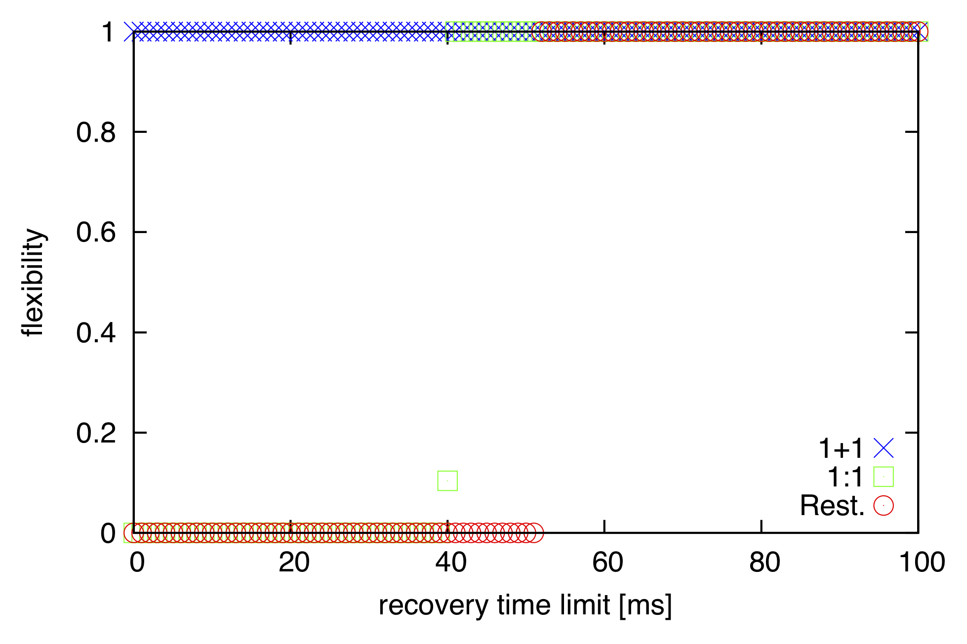
For the network flexibility evaluation, you can choose and vary the following two parameters: topology and ratio of link failures (default: Abilene with 0.0 = all single link failures and 0 percent of link-pair failures). We plot the flexibility for the three different systems that differ in their reaction to failures (1+1 protection, 1:1 protection and Restoration) over the time threshold T, which represents the recovery time limit.
Flexibility Plots
Please choose the following two parameters to see the flexibility plot (default: Abilene with 0.0).
1. Choose the topology:
Abilene Tiscali Sprintlink Germany 50
2. Choose the ratio of link-pair failures (all single link failures are always part of the request set):
0.0 0.1 0.5 0.9 1.0
Observation and Explanation
In the figure, the curves represent three different survivable routing methods: 1+1 Protection, 1:1 Protection and Restoration.1+1 Protection
The recovery time is quasi instantaneous as this approach duplicates resources (i.e., bandwidth and flow rules) in the form of a disjoint path-pair and uses them simultaneously. Hence, T_recovery = T_switching, where the switching time depends from the technology applied. We used 0 ms in the evaluation.
1:1 Protection
Reserves backup resources in advance, but they are not used to send data while the primary path is operational. Hence, failure detection and notification are required to re-route the traffic from the failed primary to the backup path. Therefore, T_recovery = T_detection + T_notify_source + T_switching, where T_detection is 40 ms using bidirectional failure detection [2]. Notifying the source and target nodes of the connection (we assume bidirectional connections following the same path in both direction) to switch from the working to the protection path is calculated with 5 μs propagation delay per km of cable [3]. We assume that switching time is negligible (0 ms) compared to the other tasks.
Restoration
No protection resources are planned and reserved until a failure occurs. Hence, the after-failure tasks are failure detection, notification of the controller, recovery path computation and deployment of the modified flow rules at every switch along the new path, formally: T_recovery = T_detection + T_notify_controller + T_calculation + T_installrules, where failure detection time is 50 ms using loss-of-signal detection [2], calculation time is set to 1 ms, while the notification of the controller and propagation delay from the controller to the switches (installing new flow rules and resend data on the new path) is calculated with 5 μs propagation delay per km of cable [3].
We selected topologies with corresponding node coordinates and distance values from the Topology Zoo [4]. We selected a random node as the controller location in each network, and investigated the following failure scenarios:- Single failures (0.0): all single link failures,
- Adjacent failures 10% (0.1): all single link failures and 10% of link-pairs with a node in common,
- Adjacent failures 50% (0.5): all single link failures and 50% of link-pairs with a node in common,
- Adjacent failures 90% (0.9): all single link failures and 90% of link-pairs with a node in common,
- Dual failures (1.0): all possible single link failures and all possible link-pair failures.
We calculated the recovery time in each failure scenario for all possible source-target pairs in the topology. For each source-target pair we considered only the failure requests, which disrupt the connection between the given end-nodes. Hence, the presented flexibility values (i.e., recoverable connections within time T) are averages for all possible service disruptions in the selected topology. The curves show the ratio of recoverable connections for the selected link-pair failure ratios, while varying T.
Conclusion
On the one hand, the additional signaling delay makes restoration less flexible for recovery times up to 50 ms, which is usually required in carrier-grade networks. However, if the recovery time threshold is above 70 ms, restoration becomes the most flexible choice in the above setting, surpassing the others, as it can recover more connections and accommodate more, practically all, link-pair failures until the topology remains connected.
On the other hand, 1+1 protection shows very high flexibility regardless of T (although with an increased bandwidth cost). This is because it provides immediate connectivity after an arbitrary single failure or after a link-pair failure which affects only the primary path owing to the simultaneous primary and backup flows. However, 1+1 protection is not flexible to recover failures affecting both the primary and backup paths.
References
- W. Kellerer and A. Basta and P. Babarczi and A. Blenk and M. He and M. Klügel and A. M. Alba, "How to Measure Network Flexibility? A Proposal for Evaluating Softwarized Networks," in IEEE Communications Magazine, vol. 56, no. 10, pp. 186-192, October 2018.
- S. Sharma, D. Staessens, D. Colle, M. Pickavet and P. Demeester, "In-band control, queuing, and failure recovery functionalities for openflow," in IEEE Network, vol. 30, no. 1, pp. 106-112, January-February 2016.
- S. Huang, C. U. Martel and B. Mukherjee, "Survivable Multipath Provisioning With Differential Delay Constraint in Telecom Mesh Networks," in IEEE/ACM Transactions on Networking, vol. 19, no. 3, pp. 657-669, June 2011.
- S. Knight, H. X. Nguyen, N. Falkner, R. Bowden and M. Roughan, "The Internet Topology Zoo," in IEEE Journal on Selected Areas in Communications, vol. 29, no. 9, pp. 1765-1775, October 2011.
Use Case: Dynamic Functional Split in the 5G RAN
Introduction
5G radio access networks (RAN) feature a partially centralized architecture, in which some of the functions belonging to the mobile processing chain are centralized into a data center, whereas the remaining functions are deployed close to the remote antennas. The more functions are centralized, the higher the user data rates, as centralized functions can easily coordinated with each other to reduce their mutual interference. Nonetheless, the capacity of the fronthaul network connecting centralized and remote units limits the feasible centralization levels.
A network operator may use a flexible functional split approach to dynamically change the centralization level, in order to provide higher data rates to the users and utilize the network resources more efficiently.
We consider the following scenario. For more details see [1].
- Scenario: dense 5G deployment at the center of a city
- Objective: maximize user data rates while keeping fairness and resource efficiency
- Network topology: tree-like fronthaul network with some redundant paths
- Different system to compare for flexibility static, slow-, and fast-adapting networks
Remember, network flexibility of a function placement and flow routing represents its ability to respond to changes in the user distribution under a time threshold T and a cost threshold C.
- Flexibility aspects: function placement and flow configuration
- Request(input to flexibility evaluation): distribution of UEs within the covered area
- Time threshold T: optimal function placement changes in the order of 0.5 to 1 minute [2]
- Cost threshold C: not considered, but recorded
A solution featuring a new function placement and flow configuration may be obsolete if it is obtained and implemented beyond T, which reflects the time between substantial changes in the user distribution.
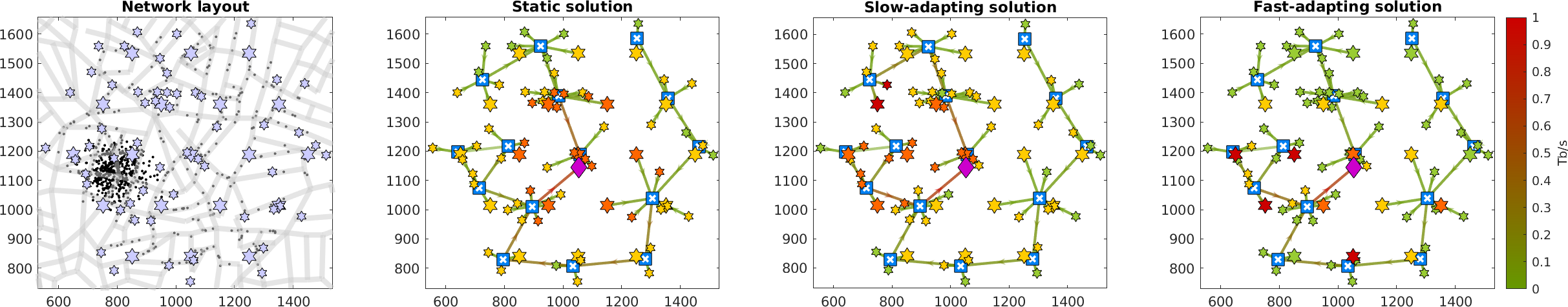
For the network flexibility evaluation, you can choose and vary the user distribution between two clusters as the time passes (1 hour in total). We show the user positions (black dots) along the location of the remote base stations (stars) in the first plot. The second, third, and fourth plots show the centralization level of each base station (green represents lowest centralization, dark red represents highest centralization) for a static, slow-adapting, and fast-adapting solution. We plot the geometric mean of the spectral efficiency achieved by the three different systems compared to the optimal values.
Flexibility Plots
Network layout
Spectral efficiency
Observations explained
Performance and network Flexibility- General trend: a slow-adapting system is able to reach near-optimal performance when the solution is fresh, but obtaining new solutions takes long (20 minutes). As a result, the performance decays until the solution is renewed, exhibitin a sawtooth behaviour. A fast-adapting solution is able to produce suboptimal solutions fast enough to feature a smooth behavior, but its performance gap is not negligible. A static solution cannot adapt to changes at all, so its performance is always substantially lower than any of the two adaptive solutions.
- Counter intuitive: Although the solutions of a slow-adapting system may decay quickly, if they are good enough the overall performance can be higher than that of a fast-adapting system. In such case, the slow-adapting network would be more flexible.
References
- A. Martinez Alba and W. Kellerer. "A Dynamic Functional Split in 5G Radio Access Networks." 2019 IEEE Global Communications Conference (GLOBECOM). IEEE, 2019.
- A. Martinez Alba, S. Janardhanan, and W. Kellerer. "Dynamics of the flexible functional split selection in 5G networks." 2020 IEEE Global Communications Conference (GLOBECOM). IEEE, 2020.